map project
Eva Koplow
2/19/2019
library(tidyverse)## ── Attaching packages ───────────────────────────────────────────────────────────────── tidyverse 1.2.1 ──## ✔ ggplot2 3.1.0 ✔ purrr 0.3.0
## ✔ tibble 2.0.1 ✔ dplyr 0.8.0.1
## ✔ tidyr 0.8.2 ✔ stringr 1.4.0
## ✔ readr 1.3.1 ✔ forcats 0.4.0## ── Conflicts ──────────────────────────────────────────────────────────────────── tidyverse_conflicts() ──
## ✖ dplyr::filter() masks stats::filter()
## ✖ dplyr::lag() masks stats::lag()library(lubridate)##
## Attaching package: 'lubridate'## The following object is masked from 'package:base':
##
## datelibrary(broom)
library(rgeos)## rgeos version: 0.4-2, (SVN revision 581)
## GEOS runtime version: 3.6.1-CAPI-1.10.1
## Linking to sp version: 1.3-1
## Polygon checking: TRUElibrary(rgdal)## Loading required package: sp## rgdal: version: 1.3-6, (SVN revision 773)
## Geospatial Data Abstraction Library extensions to R successfully loaded
## Loaded GDAL runtime: GDAL 2.1.3, released 2017/20/01
## Path to GDAL shared files: /Library/Frameworks/R.framework/Versions/3.5/Resources/library/rgdal/gdal
## GDAL binary built with GEOS: FALSE
## Loaded PROJ.4 runtime: Rel. 4.9.3, 15 August 2016, [PJ_VERSION: 493]
## Path to PROJ.4 shared files: /Library/Frameworks/R.framework/Versions/3.5/Resources/library/rgdal/proj
## Linking to sp version: 1.3-1library(maptools)## Checking rgeos availability: TRUElibrary(mapproj)## Loading required package: maps##
## Attaching package: 'maps'## The following object is masked from 'package:purrr':
##
## map# loading data files
sf_data <- read_csv("sf.csv") # it is in working directory??## Parsed with column specification:
## cols(
## Incident_Type = col_character(),
## Report_taken_date_EST = col_character(),
## Year = col_double(),
## `Data Type` = col_character(),
## Subject_Race = col_character(),
## Subject_Sex = col_character(),
## Subject_Ethnicity = col_character(),
## `Block Address` = col_character(),
## `Incident Location District` = col_character(),
## `Incident Location PSA` = col_double(),
## Age = col_character()
## )sf_data_2017 <- read_csv("sf2017.csv")## Parsed with column specification:
## cols(
## Incident_Type = col_character(),
## Report_taken_date_EST = col_character(),
## Year = col_double(),
## `Data Type` = col_character(),
## Subject_Race = col_character(),
## Subject_Sex = col_character(),
## Subject_Ethnicity = col_character(),
## `Block Address` = col_character(),
## `Incident Location District` = col_character(),
## `Incident Location PSA` = col_double(),
## Age = col_character()
## )crime <- read_csv("CrimeStatebyState.csv")## Parsed with column specification:
## cols(
## .default = col_double(),
## State = col_character()
## )## See spec(...) for full column specifications.# bind them together
sf_data <- rbind(sf_data,sf_data_2017)
# remove isolated 2017 data
remove(sf_data_2017)
# putting data into more legible categories
sf_data <- mutate(sf_data, date = mdy(Report_taken_date_EST),
Type=as.factor(`Data Type`),
Gender=as.factor(Subject_Sex),
Ethnicity=as.factor(Subject_Ethnicity),
Race=as.factor(Subject_Race),
District=as.factor(`Incident Location District`),
PSA=as.factor(`Incident Location PSA`),
Year=as.factor(Year)
)
# if age is juvenile or unknown = NA, otherwise age as numerical value
sf_data <- mutate(sf_data, num_age =
ifelse(Age=="Juvenile"|Age=="Unknown",
NA,as.numeric(Age)))## Warning in ifelse(Age == "Juvenile" | Age == "Unknown", NA,
## as.numeric(Age)): NAs introduced by coercion# cutting age into 10-year groups
sf_data <- mutate(sf_data, cat_age = cut(num_age,
breaks=c(17,27,37,47,57,67,77,87),
labels=c("18-27","28-37","38-47",
"48-57","58-67","68-77",
"78-87")))
# add "Juvenile" and "Unknown" into categorical age variable
sf_data <- mutate(sf_data, cat_age = ifelse(Age=="Juvenile"|Age=="Unknown",Age,
as.character(cat_age)))
# rename categorical age variable to Age_binned, coerce to factor
# Make "Juvenile" the first level of that factor
sf_data <- mutate(sf_data, Age_binned=as.factor(cat_age))
sf_data <- mutate(sf_data, Age=fct_relevel(Age,"Juvenile"),
Age_binned=fct_relevel(Age_binned,"Juvenile"))
# create Month variable
sf_data <- mutate(sf_data, Month=month(date,label=T,abbr=F))
# import geospatial data about Police Districts
districts <- readOGR("Police_Districts.shp",layer="Police_Districts")## OGR data source with driver: ESRI Shapefile
## Source: "/Users/evakoplow/Desktop/portfolio_koplow/Police_Districts.shp", layer: "Police_Districts"
## with 7 features
## It has 8 fields
## Integer64 fields read as strings: OBJECTID DISTRICT# defining districts as "id" variable
names(districts@data)[1] <- "id"
# extracting the lat/long coordinates of district boundary points
# telling the tidy function that the region value can be found in the "id" variable
districts.points <- tidy(districts, region="id")## Warning in bind_rows_(x, .id): Unequal factor levels: coercing to character## Warning in bind_rows_(x, .id): binding character and factor vector,
## coercing into character vector
## Warning in bind_rows_(x, .id): binding character and factor vector,
## coercing into character vector
## Warning in bind_rows_(x, .id): binding character and factor vector,
## coercing into character vector
## Warning in bind_rows_(x, .id): binding character and factor vector,
## coercing into character vector
## Warning in bind_rows_(x, .id): binding character and factor vector,
## coercing into character vector
## Warning in bind_rows_(x, .id): binding character and factor vector,
## coercing into character vector
## Warning in bind_rows_(x, .id): binding character and factor vector,
## coercing into character vector# combine lat/long coordinates of district boundary points with data about districts
districts.cart <- full_join(districts.points, districts@data, by="id")## Warning: Column `id` joining character vector and factor, coercing into
## character vector# import geospatial data about Police Service Areas
psas <- readOGR("Police_Service_Areas.shp",layer="Police_Service_Areas")## OGR data source with driver: ESRI Shapefile
## Source: "/Users/evakoplow/Desktop/portfolio_koplow/Police_Service_Areas.shp", layer: "Police_Service_Areas"
## with 56 features
## It has 24 fields
## Integer64 fields read as strings: OBJECTID DISTRICT PSA TOTALPOP WHITE BLACK NAT_AMER ASIAN OTHER TWO_ORMORE HISPANIC POPMALE POPFEMALE POPUNDER18 POP65UP# extracting the lat/long coordinates of PSA boundary points
# telling the tidy function that the region value can be found in the "PSA" variable
psas.points <- tidy(psas, region="PSA")## Warning in bind_rows_(x, .id): Unequal factor levels: coercing to character
## Warning in bind_rows_(x, .id): binding character and factor vector,
## coercing into character vector

## Warning in bind_rows_(x, .id): binding character and factor vector,
## coercing into character vector

## Warning in bind_rows_(x, .id): binding character and factor vector,
## coercing into character vector

## Warning in bind_rows_(x, .id): binding character and factor vector,
## coercing into character vector

## Warning in bind_rows_(x, .id): binding character and factor vector,
## coercing into character vector

## Warning in bind_rows_(x, .id): binding character and factor vector,
## coercing into character vector

## Warning in bind_rows_(x, .id): binding character and factor vector,
## coercing into character vector
## Warning in bind_rows_(x, .id): binding character and factor vector,
## coercing into character vector
## Warning in bind_rows_(x, .id): binding character and factor vector,
## coercing into character vector
## Warning in bind_rows_(x, .id): binding character and factor vector,
## coercing into character vector
## Warning in bind_rows_(x, .id): binding character and factor vector,
## coercing into character vector
## Warning in bind_rows_(x, .id): binding character and factor vector,
## coercing into character vector
## Warning in bind_rows_(x, .id): binding character and factor vector,
## coercing into character vector
## Warning in bind_rows_(x, .id): binding character and factor vector,
## coercing into character vector
## Warning in bind_rows_(x, .id): binding character and factor vector,
## coercing into character vector
## Warning in bind_rows_(x, .id): binding character and factor vector,
## coercing into character vector
## Warning in bind_rows_(x, .id): binding character and factor vector,
## coercing into character vector
## Warning in bind_rows_(x, .id): binding character and factor vector,
## coercing into character vector
## Warning in bind_rows_(x, .id): binding character and factor vector,
## coercing into character vector
## Warning in bind_rows_(x, .id): binding character and factor vector,
## coercing into character vector
## Warning in bind_rows_(x, .id): binding character and factor vector,
## coercing into character vector
## Warning in bind_rows_(x, .id): binding character and factor vector,
## coercing into character vector
## Warning in bind_rows_(x, .id): binding character and factor vector,
## coercing into character vector
## Warning in bind_rows_(x, .id): binding character and factor vector,
## coercing into character vector
## Warning in bind_rows_(x, .id): binding character and factor vector,
## coercing into character vector
## Warning in bind_rows_(x, .id): binding character and factor vector,
## coercing into character vector
## Warning in bind_rows_(x, .id): binding character and factor vector,
## coercing into character vector
## Warning in bind_rows_(x, .id): binding character and factor vector,
## coercing into character vector
## Warning in bind_rows_(x, .id): binding character and factor vector,
## coercing into character vector
## Warning in bind_rows_(x, .id): binding character and factor vector,
## coercing into character vector
## Warning in bind_rows_(x, .id): binding character and factor vector,
## coercing into character vector
## Warning in bind_rows_(x, .id): binding character and factor vector,
## coercing into character vector
## Warning in bind_rows_(x, .id): binding character and factor vector,
## coercing into character vector
## Warning in bind_rows_(x, .id): binding character and factor vector,
## coercing into character vector
## Warning in bind_rows_(x, .id): binding character and factor vector,
## coercing into character vector
## Warning in bind_rows_(x, .id): binding character and factor vector,
## coercing into character vector
## Warning in bind_rows_(x, .id): binding character and factor vector,
## coercing into character vector
## Warning in bind_rows_(x, .id): binding character and factor vector,
## coercing into character vector
## Warning in bind_rows_(x, .id): binding character and factor vector,
## coercing into character vector
## Warning in bind_rows_(x, .id): binding character and factor vector,
## coercing into character vector
## Warning in bind_rows_(x, .id): binding character and factor vector,
## coercing into character vector
## Warning in bind_rows_(x, .id): binding character and factor vector,
## coercing into character vector
## Warning in bind_rows_(x, .id): binding character and factor vector,
## coercing into character vector
## Warning in bind_rows_(x, .id): binding character and factor vector,
## coercing into character vector
## Warning in bind_rows_(x, .id): binding character and factor vector,
## coercing into character vector
## Warning in bind_rows_(x, .id): binding character and factor vector,
## coercing into character vector
## Warning in bind_rows_(x, .id): binding character and factor vector,
## coercing into character vector
## Warning in bind_rows_(x, .id): binding character and factor vector,
## coercing into character vector
## Warning in bind_rows_(x, .id): binding character and factor vector,
## coercing into character vector
## Warning in bind_rows_(x, .id): binding character and factor vector,
## coercing into character vector
## Warning in bind_rows_(x, .id): binding character and factor vector,
## coercing into character vector
## Warning in bind_rows_(x, .id): binding character and factor vector,
## coercing into character vector
## Warning in bind_rows_(x, .id): binding character and factor vector,
## coercing into character vector
## Warning in bind_rows_(x, .id): binding character and factor vector,
## coercing into character vector
## Warning in bind_rows_(x, .id): binding character and factor vector,
## coercing into character vector
## Warning in bind_rows_(x, .id): binding character and factor vector,
## coercing into character vector# combine lat/long coordinates of district boundary points with data about districts
# tell join function that "id" in psas.points corresponds to "PSA" in psas@data
psas.cart <- full_join(psas.points, psas@data, by=c("id" = "PSA"))## Warning: Column `id`/`PSA` joining character vector and factor, coercing
## into character vectorplot_data <- filter(sf_data,!is.na(PSA))
all_cats <- expand(plot_data,PSA,Subject_Sex)
plot_data <- summarize(group_by(plot_data, PSA,Subject_Sex),reports=n())
plot_data <- full_join(plot_data,all_cats,by=c("PSA","Subject_Sex"))
#plot_data <- mutate(plot_data,reports=replace_na(reports,0))
names(plot_data)[1] <- "NAME"
mapdata <- full_join(plot_data,psas.cart,by="NAME")
g <- ggplot() +
geom_polygon(data=drop_na(mapdata), aes(x=long, y=lat, group=group,fill=reports),color="black") +
coord_map()+
theme_void()
g+facet_wrap(~Subject_Sex)+
scale_fill_distiller(palette="Spectral", name="Number of Reports")+
labs(title="SF Reports in Police Service Areas Faceted by Gender")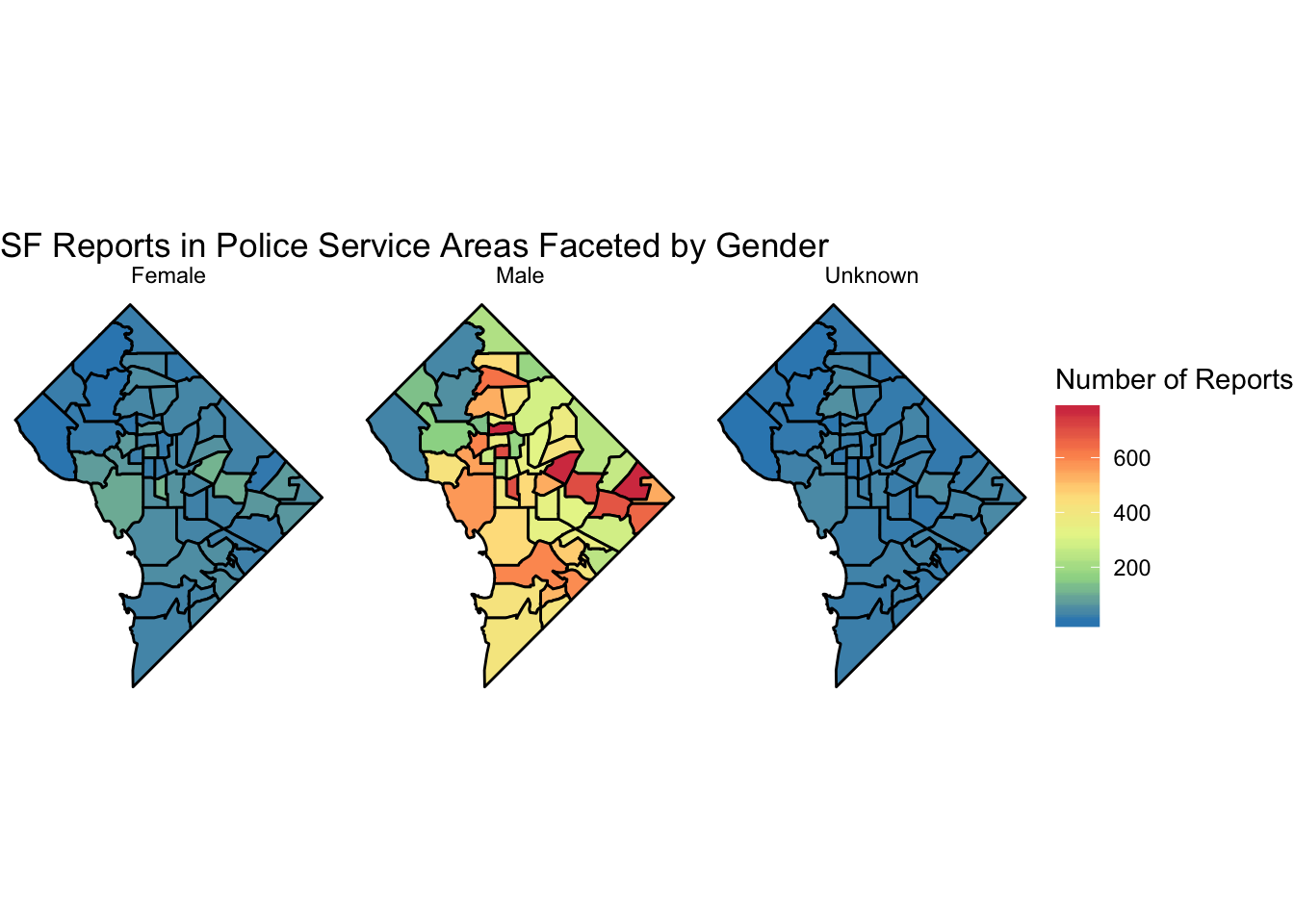
plot2_data <- filter(sf_data,!is.na(District))

levels(plot2_data$District) <- c("First District","Second District",
                                "Third District","Fourth District",
                                "Fifth District","Sixth District",
                                "Seventh District")

all_cats <- expand(plot2_data,District,Age_binned)

plot2_data <- summarize(group_by(plot2_data, District,Age_binned),reports=n())
## Warning: Factor `Age_binned` contains implicit NA, consider using
## `forcats::fct_explicit_na`plot2_data <- full_join(plot2_data,all_cats,by=c("District","Age_binned"))
#plot_data <- mutate(plot_data,reports=replace_na(reports,0))
names(plot2_data)[1] <- "NAME"
mapdata <- full_join(plot2_data,districts.cart,by="NAME")## Warning: Column `NAME` joining factors with different levels, coercing to
## character vectorg <- ggplot() +
geom_polygon(data=mapdata,
aes(x=long, y=lat, group=group,fill=reports),color="black") +
coord_map()+
theme_void()
g+facet_wrap(~Age_binned)+
scale_fill_distiller(palette="Spectral", name="Number of Reports",na.value="white")+
labs(title="SF Reports in Police Districts Faceted by Age Group")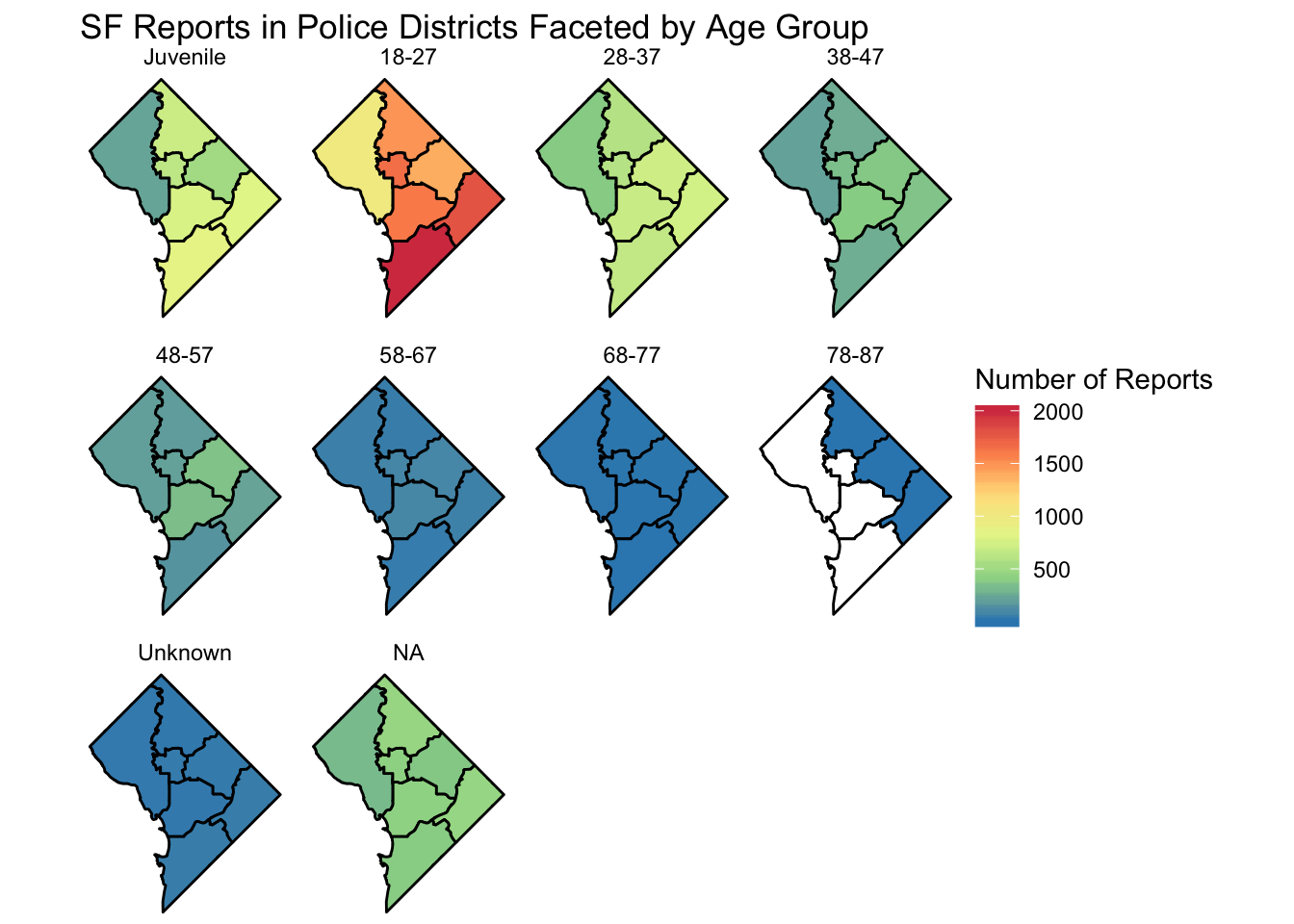
us_data <- filter(crime, State=="United States-Total")

ggplot(us_data) + geom_line(aes(x=Year, y=`Violent Crime rate`), color="green")+
  labs(title="Violent Crime Rate in the US", x="Year", Y="Violent Crime Rate")+
  theme_classic()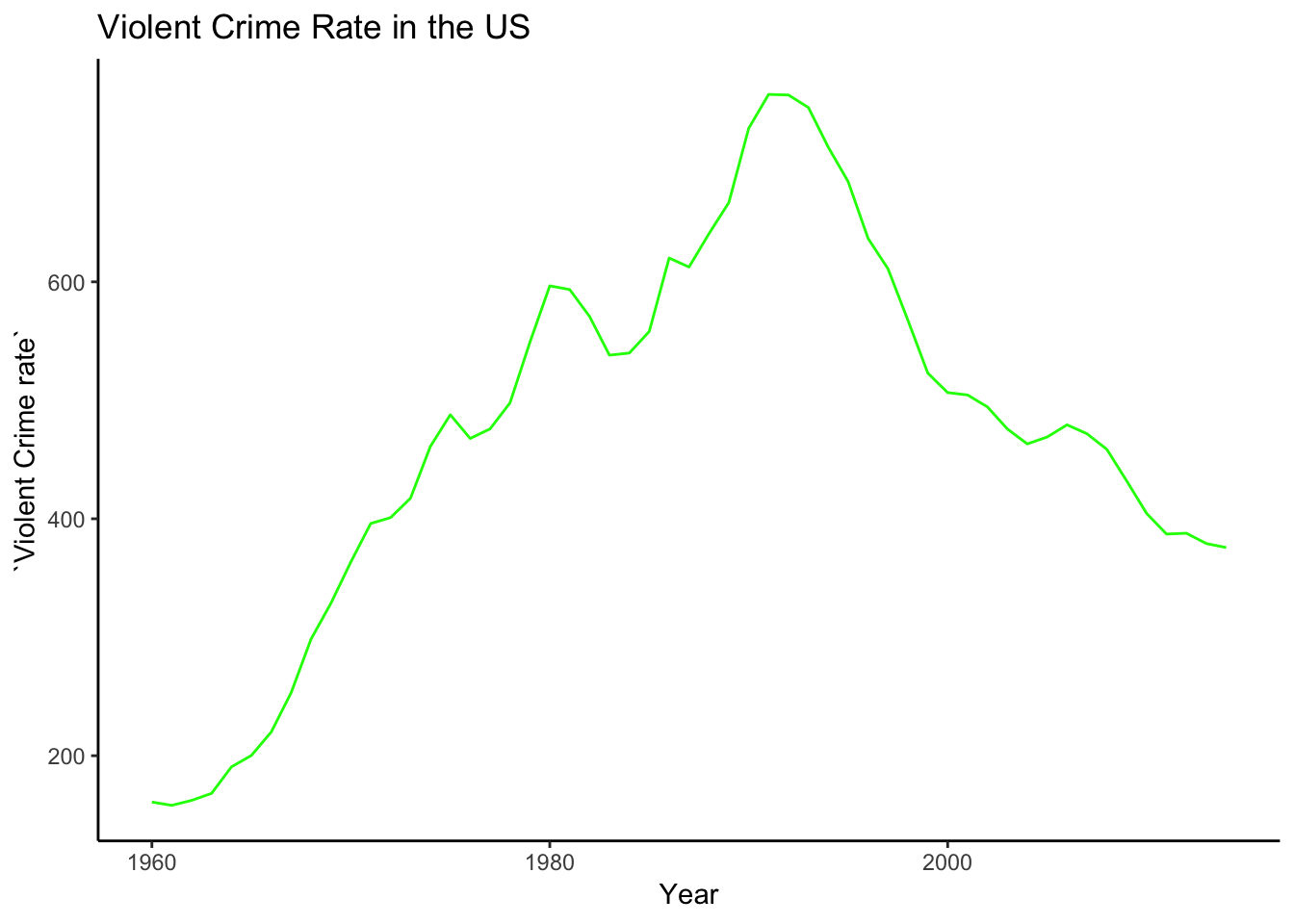
us_4_crimes <- select(us_data, Year, `Aggravated assault rate`,
                      `Murder and nonnegligent manslaughter rate`,
                      `Legacy rape rate /1`,`Robbery rate`)
us_4_crimes_plot <- gather(us_4_crimes, key="Violent Crime Type",
                           value= Rate, `Aggravated assault rate`:`Robbery rate`)
ggplot(us_4_crimes_plot) + geom_line(aes(x=Year, y= Rate, color=`Violent Crime Type`))+
  scale_color_discrete(name="Type of Violent Crime",
                       labels=c("Aggravated Assault","Rape", "Murder and Nonnegligent Manslaughter","Robbery"))+theme_classic()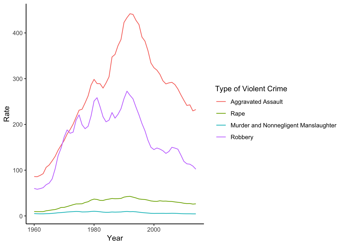
state_crime <- filter(crime, State!="United States-Total")

northeast_states<- c("Connecticut", "Maine", "Massachusetts", "New Hampshire", "Rhode Island", "Vermont", "New Jersey", "New York", "Pennsylvania")
midwest_states <- c("Illinois", "Indiana", "Michigan", "Ohio", "Wisconsin", "Iowa", "Kansas", "Minnesota", "Missouri", "Nebraska", "North Dakota", "South Dakota")
south_states <- c("Delaware", "Florida", "Georgia", "Maryland", "North Carolina", "South Carolina", "Virginia", "District of Columbia", "West Virginia", "Alabama", "Kentucky", "Mississippi", "Tennessee", "Arkansas", "Louisiana", "Oklahoma", "Texas")
west_states <- c("Arizona", "Colorado", "Idaho", "Montana", "Nevada", "New Mexico", "Utah", "Wyoming", "Alaska", "California", "Hawaii", "Oregon", "Washington")

state_crime <- mutate(state_crime, region=ifelse(State %in% northeast_states, "Northeast",
                                                 ifelse(State %in% midwest_states, "Midwest",
                                                        ifelse(State %in% south_states, "South",
                                                               ifelse(State %in% west_states, "West","NA")))))

regional_rates <- summarize(group_by(state_crime, region, Year),
                            `Property crime rate`=
                              sum(`Property crime total`)/sum(Population)*100000)

ggplot(regional_rates) + geom_line(aes(x=Year, y=`Property crime rate`, color=region))+labs(title="Overall Property Crime Rate for the 4 Census Regions")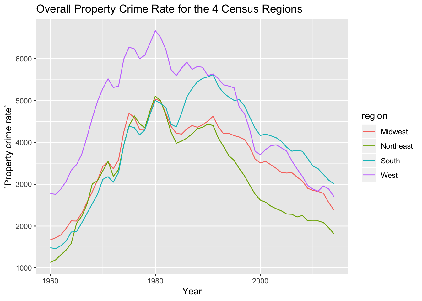
crime_2013 <- filter(crime, Year==2013, State!="United States-Total")
all_states <- map_data("state")

crime_2013 <- rename(crime_2013,region=State)
crime_2013 <- mutate(crime_2013, region=tolower(region))

stateData <- left_join(all_states,crime_2013,by="region")

ggplot()+
  geom_polygon(data=stateData,
               aes(x=long, y=lat, group = group,
                   fill=`Robbery rate`),
               color="grey50")+
  scale_fill_distiller(palette="Oranges", direction=1)+
  coord_map()+labs(title="Robbery Rate in 2013")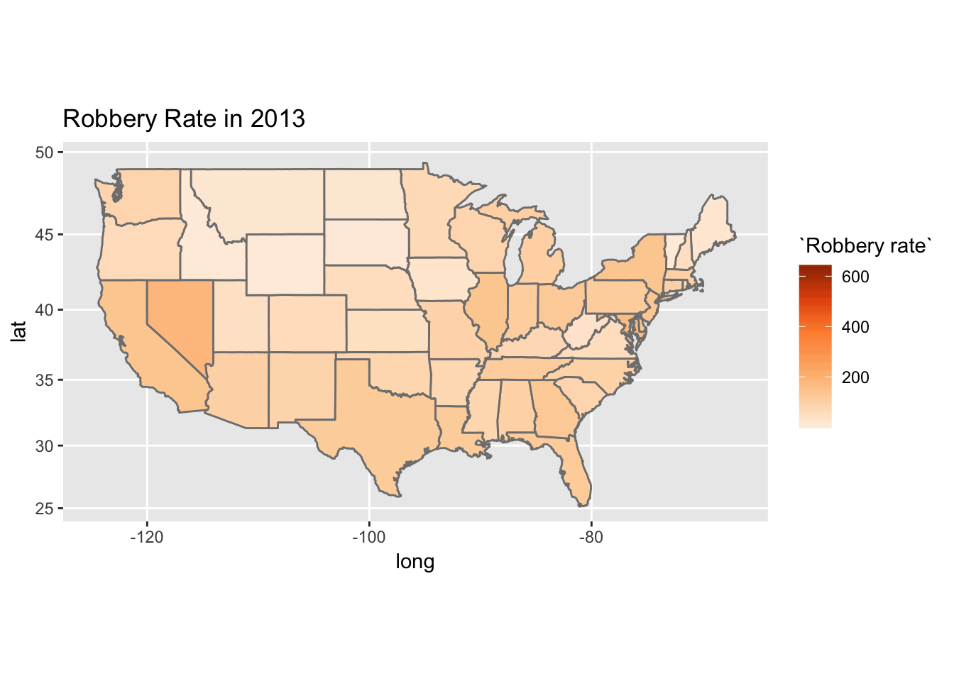
library(treemap) # ask professor meyer
crime_2010 <- filter(crime, Year==2010, State!="United States-Total")
treemap(crime_2013,index="region",
        vSize="Population",
        vColor="Murder and nonnegligent manslaughter rate",
        type="value",palette="Reds")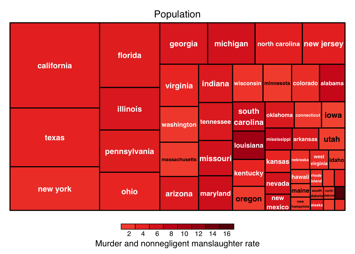
crime_1990 <- filter(crime, Year==1990, State!="United States-Total")
northeast_states<- c("Connecticut", "Maine", "Massachusetts", "New Hampshire", "Rhode Island", "Vermont", "New Jersey", "New York", "Pennsylvania")
midwest_states <- c("Illinois", "Indiana", "Michigan", "Ohio", "Wisconsin", "Iowa", "Kansas", "Minnesota", "Missouri", "Nebraska", "North Dakota", "South Dakota")
south_states <- c("Delaware", "Florida", "Georgia", "Maryland", "North Carolina", "South Carolina", "Virginia", "District of Columbia", "West Virginia", "Alabama", "Kentucky", "Mississippi", "Tennessee", "Arkansas", "Louisiana", "Oklahoma", "Texas")
west_states <- c("Arizona", "Colorado", "Idaho", "Montana", "Nevada", "New Mexico", "Utah", "Wyoming", "Alaska", "California", "Hawaii", "Oregon", "Washington")

crime_1990 <- mutate(crime_1990, region=ifelse(State %in% northeast_states, "Northeast",
                                                 ifelse(State %in% midwest_states, "Midwest",
                                                        ifelse(State %in% south_states, "South",
                                                               ifelse(State %in% west_states, "West","NA")))))


ggplot(crime_1990)+geom_point(aes(x=`Motor vehicle theft rate`,
                                  y=`Burglary rate`,
                                  color=region,
                                  shape=region))+
  scale_shape_manual(values=c("Midwest"=2,"Northeast"=5,"South"=0,"West"=1))+scale_color_manual(values=c("Midwest"="purple", "Northeast"="blue", "South"="green", "West"="red"))+
      labs(x="Motor Vehicle Theft Rate", y="Burglary Rate", title="Burglary Rate in 1990 vs. Vehicle Theft Rate in 1990")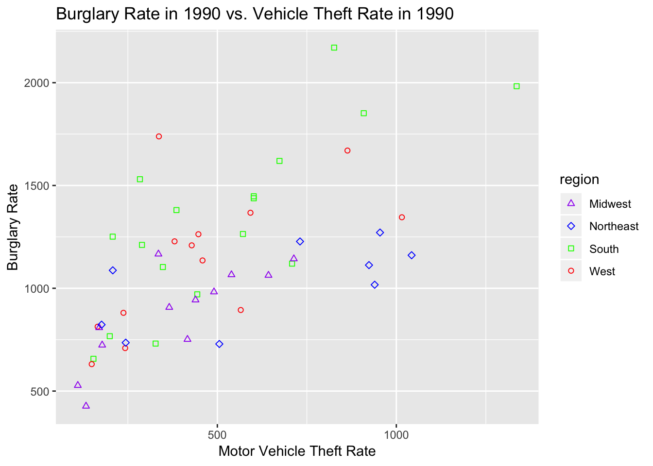
crime_2014 <- filter(crime, Year==2014, State!="United States-Total")

ggplot(crime_2014)+geom_point(aes(x=`Larceny-theft rate`,
                                  y=`Aggravated assault rate`,
                                  #color=State,
                                  size=Population))+
                                scale_fill_manual(values=c("Midwest"="purple", "Northeast"="blue", "South"="green", "West"="red"))+
      labs(x="Larceny Theft Rate", y="Burglary Rate", title="Larceny Theft Rate in 2014 vs. Aggravated Assault Rate in 2014")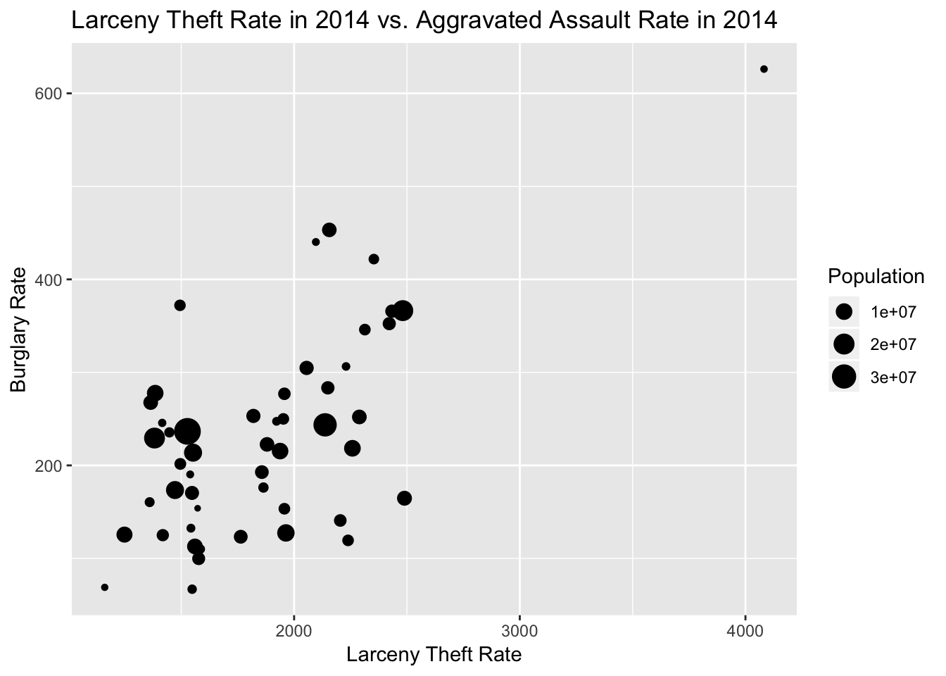
library(tidyverse)
library(tidyverse)
diamonds.small <-  diamonds[sample(nrow(diamonds), 500),]

q <- ggplot(diamonds.small,aes(x=carat, y=price))

########GRAPH 1#############
q + geom_point() #scatter plot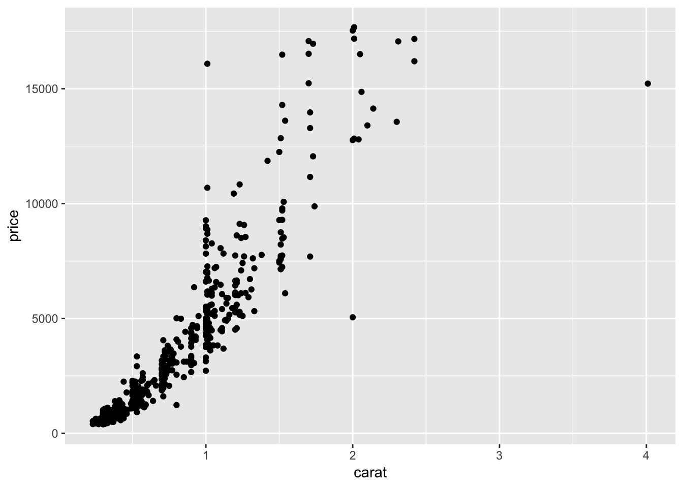
########GRAPH 2 ################
q + geom_count(aes(size=..prop..),alpha=.5) #bubble plot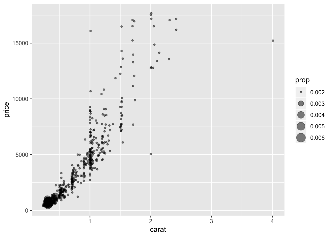
########GRAPH 3 ################
q <- ggplot(diamonds.small,aes(x=carat, y=price))
q + geom_count(aes(size=..prop..,color=as.factor(cut)),alpha=.5) #bubble plot
########GRAPH 4 ################
q + geom_bin2d()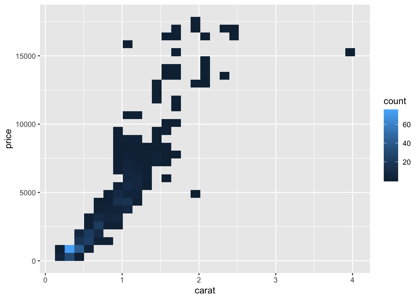
########GRAPH 5 ################
q + stat_density2d() +
  scale_x_continuous(lim=c(-.3,4.0)) +
  scale_y_continuous(lim=c(-8000,18900))
## Warning: Removed 1 rows containing non-finite values (stat_density2d).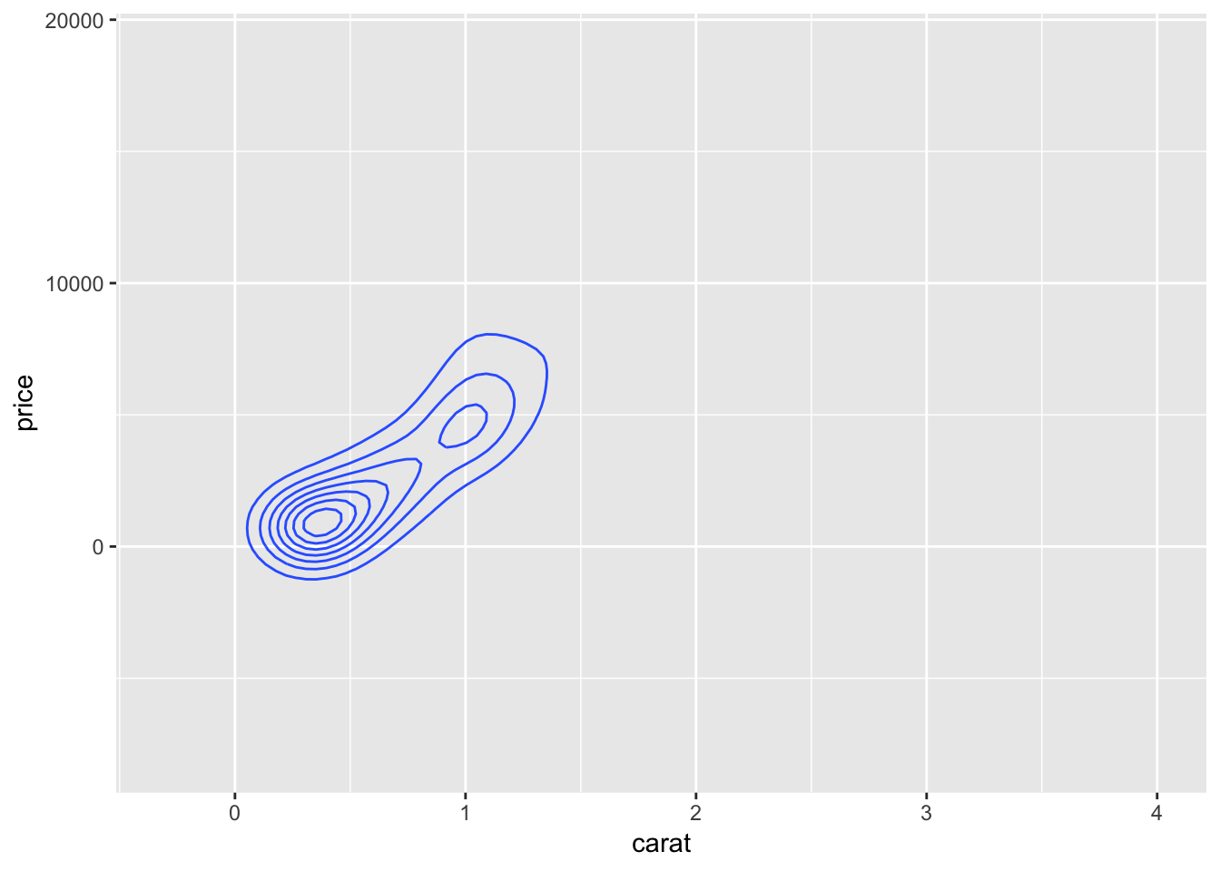
########GRAPH 6 ################

q + geom_jitter() + geom_smooth(method = "lm", se=T, level=.95)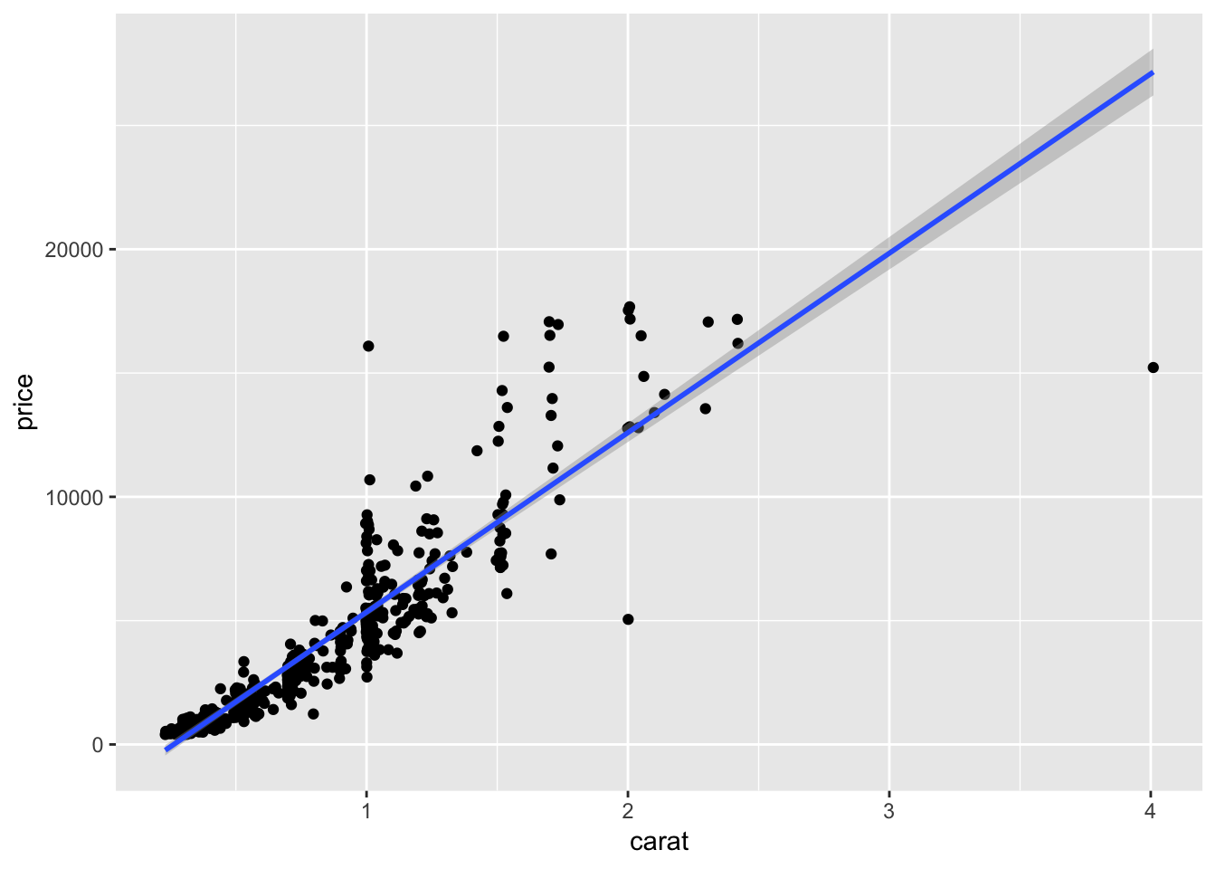
########GRAPH 7 ################
ggplot(diamonds.small,aes(x=carat, y=price,color=as.factor(cut)),alpha=.5 )+ geom_jitter() + geom_smooth(method = "lm", se=T, level=.67)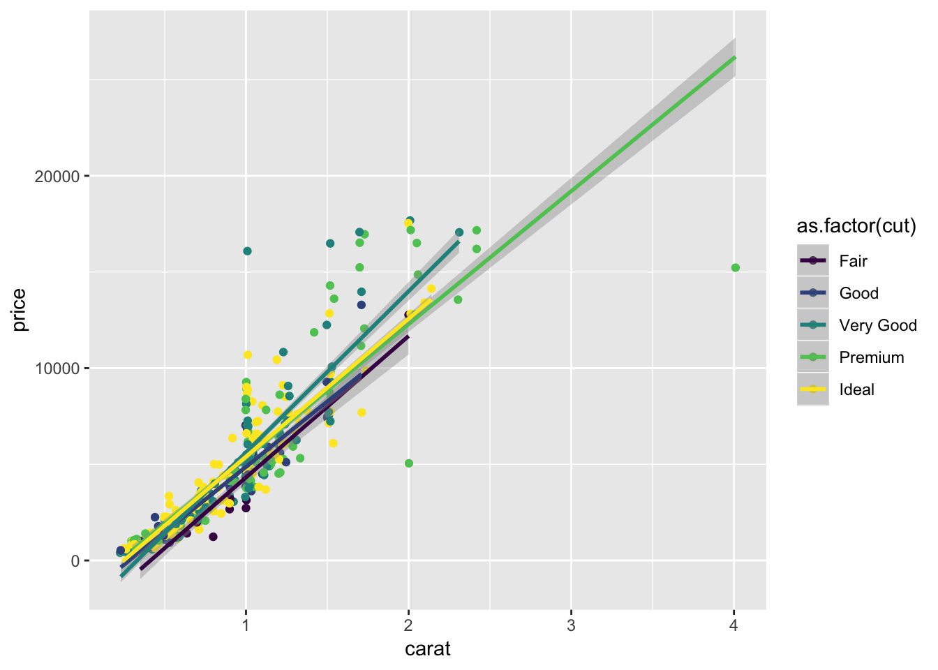
########GRAPH 8 ################
ggplot(diamonds.small,aes(x=carat, y=price,color=as.factor(cut)),alpha=.5 )+ geom_jitter() + geom_smooth(method = "lm",formula=y~poly(x,2))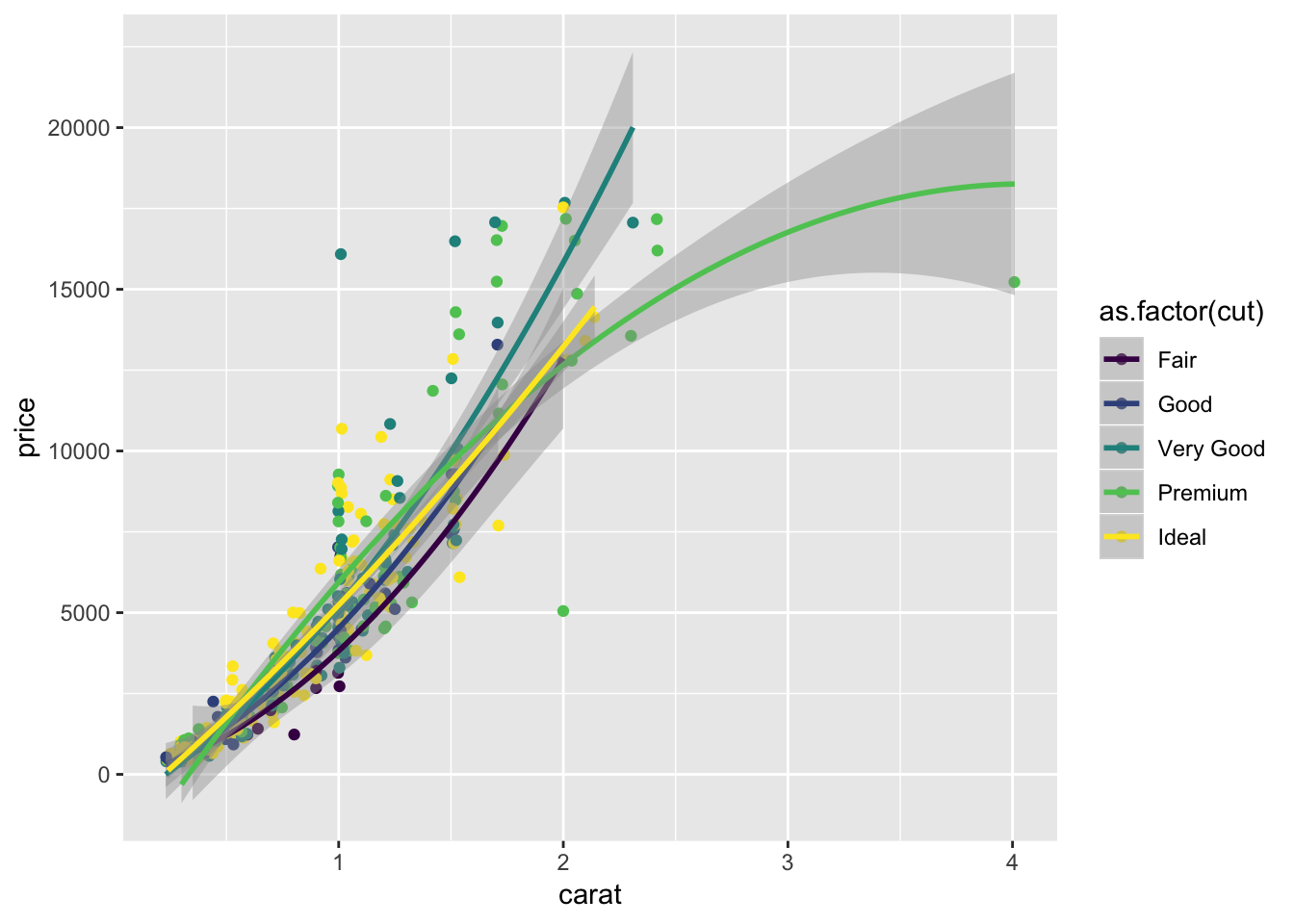 These graphs were created using the diamonds dataset in the ggplot2 library. The first few graphs show how to create a scatterplot of carat vs. price and a bubble plot of carat vs. price where the size of the point is representative of its frequency. The last few graphs illustrate a jittered scatterplot with trendlines. The goal of these visualizations is to examine correlations between diamond carat and price. The graphs all show that as carat increases, so does price.